The AR1 model, also known as the Autoregressive model of order 1, is a statistical model used to forecast and analyze time series data. It is a simple yet powerful tool for understanding and predicting patterns in data that vary over time. In this article, we will delve into the specifics of the AR1 model, its applications, and provide 5 tips for effectively using this model in real-world scenarios.
Key Points
- Understanding the basics of the AR1 model and its formulation
- Choosing the right data for AR1 model application
- Estimating model parameters with precision
- Interpreting results and forecasting with the AR1 model
- Addressing limitations and potential pitfalls of the AR1 model
Introduction to the AR1 Model

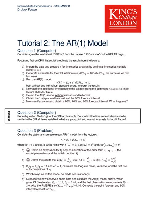
The AR1 model is based on the principle that the current value of a time series can be predicted using a linear combination of past values, plus an error term. Mathematically, it is represented as (Y_t = \beta_0 + \beta1 Y{t-1} + \epsilon_t), where (Y_t) is the value at time (t), (\beta_0) is the constant term, (\beta_1) is the coefficient of the lagged term, and (\epsilon_t) is the error term at time (t). This model is particularly useful for time series that exhibit strong autocorrelation, meaning that the current value is significantly influenced by the immediately preceding value.
Tip 1: Understanding the Basics and Formulation
Before applying the AR1 model, it’s crucial to understand its formulation and the assumptions it makes about the data. The model assumes that the time series is stationary, meaning that the mean, variance, and autocorrelation structure remain constant over time. Non-stationarity can often be addressed through differencing or transformation of the data. Furthermore, understanding how to estimate the model parameters ((\beta_0) and (\beta_1)) and how to interpret them is essential for meaningful analysis and forecasting.
Applications and Data Selection

The choice of data is critical when applying the AR1 model. It is most appropriately used with time series data that shows a strong and consistent pattern of autocorrelation. Economic indicators, stock prices, and weather patterns are examples of data that might be suitable for AR1 modeling, provided they exhibit the necessary autocorrelative structure. It’s also important to ensure that the data is properly cleaned and preprocessed to remove any anomalies or trends that could distort the model’s accuracy.
Tip 2: Choosing the Right Data
Not all time series data is suitable for the AR1 model. Data with strong seasonal components, for instance, may require more complex models like SARIMA (Seasonal ARIMA) to accurately capture the seasonal patterns. Similarly, data with trends may need differencing to make it stationary before applying the AR1 model. Therefore, careful analysis of the data’s characteristics, including tests for stationarity and autocorrelation, is a prerequisite for successful application of the AR1 model.
Estimating Model Parameters
Estimating the parameters of the AR1 model, particularly (\beta_1), is crucial for the model’s predictive power. The most common method for estimating these parameters is ordinary least squares (OLS) regression, which minimizes the sum of the squared errors to find the best-fit line. However, it’s essential to check for the assumptions of OLS, such as no serial correlation in the residuals and homoscedasticity, to ensure the validity of the estimates.
Tip 3: Estimating Model Parameters with Precision
Using diagnostic tests such as the Durbin-Watson test for serial correlation and plotting the residuals against time or the fitted values can help in identifying any violations of the OLS assumptions. If violations are found, alternative estimation methods or transformations of the data may be necessary. Additionally, considering the use of information criteria (AIC, BIC) can help in selecting the most appropriate model among different specifications.
Interpreting Results and Forecasting
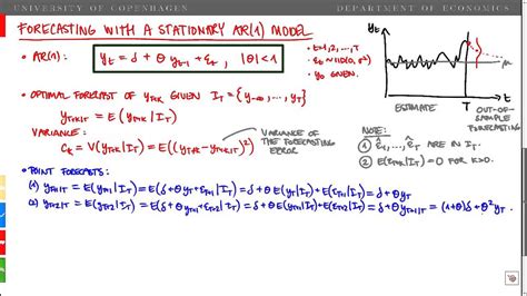
Once the model parameters are estimated, the AR1 model can be used to make forecasts. The forecast for the next period is made by plugging the last observed value into the model equation. For multi-step ahead forecasts, the process is iterative, using the forecasted value as the input for the next period’s forecast. Understanding how to interpret these forecasts, including calculating forecast intervals to quantify uncertainty, is vital for decision-making.
Tip 4: Interpreting Results and Forecasting
It’s also important to monitor the performance of the AR1 model over time, using metrics such as mean absolute error (MAE) or mean squared error (MSE), to assess its accuracy. If the model’s performance deteriorates, re-estimation of the parameters or consideration of alternative models may be necessary. Moreover, combining the AR1 model with other forecasting techniques, such as exponential smoothing or machine learning models, can sometimes improve forecasting accuracy through ensemble methods.
Addressing Limitations and Potential Pitfalls

While the AR1 model is a powerful tool for time series analysis, it has its limitations. It assumes a linear relationship between the current and past values, which may not always be the case. Non-linear relationships or the presence of outliers can significantly affect the model’s performance. Additionally, the model’s simplicity means it may not capture more complex patterns or structures in the data, such as seasonality or trends, without additional preprocessing or model extensions.
Tip 5: Addressing Limitations and Potential Pitfalls
Being aware of these limitations and taking steps to address them is crucial. This might involve exploring more complex models that can accommodate non-linearities or seasonal patterns, or using robust estimation methods that are less affected by outliers. Continuous monitoring of the model’s performance and a willingness to adapt or change the model as necessary are key to successfully applying the AR1 model in real-world applications.
What is the primary assumption of the AR1 model?
+The primary assumption of the AR1 model is that the time series is stationary, meaning that the mean, variance, and autocorrelation structure remain constant over time.
How do you estimate the parameters of the AR1 model?
+The parameters of the AR1 model are commonly estimated using ordinary least squares (OLS) regression, which minimizes the sum of the squared errors to find the best-fit line.
What are some limitations of the AR1 model?
+The AR1 model assumes a linear relationship between the current and past values and may not capture more complex patterns or structures in the data, such as seasonality or trends, without additional preprocessing or model extensions.
In conclusion, the AR1 model is a valuable tool for time series analysis and forecasting, offering insights into the autocorrelative structure of data. By understanding its formulation, choosing the right data, estimating model parameters with precision, interpreting results for forecasting, and addressing its limitations, practitioners can effectively leverage the AR1 model to make informed decisions in a variety of fields. Continuous learning and adaptation, considering the evolving nature of time series data and the development of new analytical techniques, are essential for maximizing the utility of the AR1 model in real-world applications.


